Insertion Sort Algorithm

Ever Wondered How Insertion Sort Efficiently Organizes Data? Let’s Dive In!

Sorting data might seem like a mundane task, but when you understand the algorithms behind it, it becomes a fascinating process. One of the simplest yet effective algorithms is Insertion Sort. Whether you’re a programmer trying to optimize your code or a student learning data structures, mastering Insertion Sort can open up a world of possibilities.

But how exactly does it work? Why is it called “insertion,” and how can it be applied in real-world scenarios? Let’s break it down step by step!

What is Insertion Sort and Why Does it Matter?

At its core, Insertion Sort is a simple comparison-based algorithm that builds the final sorted array one item at a time. The beauty of this approach lies in how each new element is placed in its correct position, just like sorting a deck of cards. Imagine starting with a hand of unsorted cards and picking them up one by one, inserting each in its appropriate position relative to the already sorted cards.

This algorithm shines when you’re working with smaller datasets or partially sorted arrays. But why is it so important in the world of algorithms?

For many programmers and computer scientists, Insertion Sort serves as a stepping stone to understanding more complex algorithms, like Merge Sort or Quick Sort. It is intuitive, easy to implement, and, most importantly, offers insight into data manipulation at a fundamental level.

 Key Concepts Behind Insertion Sort

1. How It Works

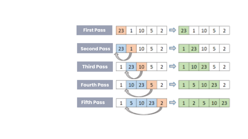
Insertion Sort operates by iterating over an array, starting from the second element. For each element, it is compared with elements before it. If the current element is smaller, it is shifted to the correct position by swapping it backward in the array.

2. Breaking It Down Step-by-Step

Here’s a step-by-step look at how Insertion Sort works:

• Start with the second element in the array (because the first element is trivially “sorted”).
• Compare this element with the one before it.
• If it is smaller, swap it.
• Continue this process with each subsequent element until the entire array is sorted.

Example: Consider the array: {13, 46, 24, 52, 20, 9}.

• Start with 46 (second element). Since 46 > 13, no change is needed.
• Move to 24. Since 24 < 46, swap them. Now, the array looks like {13, 24, 46, 52, 20, 9}.
• Move to 52. Since 52 > 46, no change is needed.
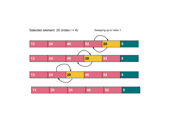
• Move to 20. Swap it backward until it reaches its correct position: {13, 20, 24, 46, 52, 9}.
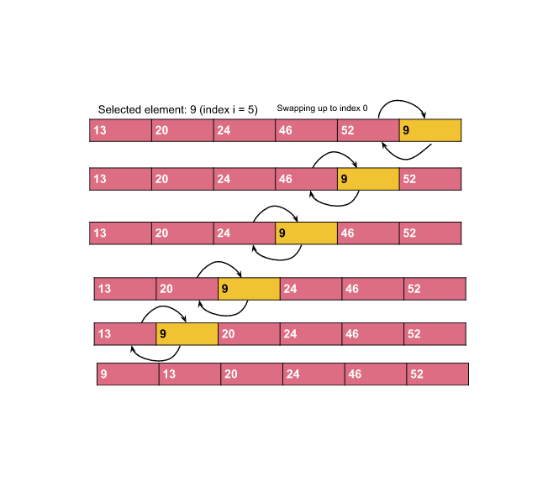
• Finally, place 9 in the correct spot after shifting: {9, 13, 20, 24, 46, 52}.

By the end of these steps, the array is fully sorted.

3. Time and Space Complexity

• Worst-case time complexity: O(n²), where n is the number of elements. This happens when the array is sorted in reverse order, requiring each new element to be compared with every previous element.
• Best-case time complexity: O(n), when the array is already sorted. In this case, no swaps are needed, and each element is compared only once.
• Space complexity: O(1), as Insertion Sort works in-place, requiring no additional storage beyond the input array.

Here’s how Insertion Sort works, step-by-step:

1. Start with the first element – Consider the first element as already sorted (since a single element is always “sorted”).
2. Pick the next element – Take the next element and compare it with the previous elements.
3. Place it in the right position – Keep shifting elements that are larger than the picked element to the right and place the picked element in its correct position.
4. Repeat – Move to the next element and repeat the process until all elements are sorted.

Now, let’s look at an example to make things clearer.

Sorting an Array with Insertion Sort

Input:
Array: {13, 46, 24, 52, 20, 9}
Output:
Sorted Array: {9, 13, 20, 24, 46, 52}

Let’s break down how Insertion Sort would sort this array step-by-step:

• Step 1: Start with the first element (13). Since it’s the only element, it’s already considered sorted.

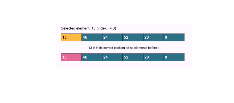
• Step 2: Move to the next element, 46. Since 46 is greater than 13, we don’t need to move anything. The sorted array is now {13, 46}.

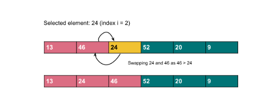
• Step 3: Move to the next element, 24. Now, compare 24 with 46 and 13. Since 24 is smaller than 46, we swap them. Now the array looks like {13, 24, 46}.

• Step 4: Move to 52. Since 52 is larger than all the elements in the sorted portion, no swapping is needed. The sorted array is now {13, 24, 46, 52}.

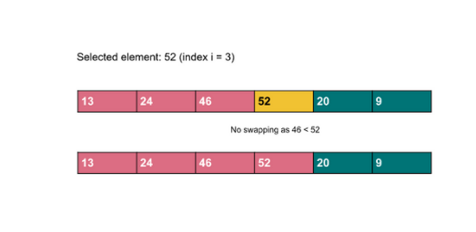
• Step 5: Move to 20. Compare 20 with 52, 46, and 24. It’s smaller than all of them, so we keep shifting them to the right and place 20 between 13 and 24. The array is now {13, 20, 24, 46, 52}.

• Step 6: Finally, move to 9. It’s smaller than all the elements, so we keep shifting everything to the right and place 9 at the beginning. The final sorted array is {9, 13, 20, 24, 46, 52}.

That’s it! In just six steps, you have a fully sorted array using Insertion Sort.

#include <bits/stdc++.h>
using namespace std;

void insertion_sort(int arr[], int n) {
    for (int i = 0; i <= n - 1; i++) {
        int j = i;
        while (j > 0 && arr[j - 1] > arr[j]) {
            int temp = arr[j - 1];
            arr[j - 1] = arr[j];
            arr[j] = temp;
            j--;
        }
    }

    cout << "After Using insertion sort: " << "\n";
    for (int i = 0; i < n; i++) {
        cout << arr[i] << " ";
    }
    cout << "\n";
}

int main()
{
    int arr[] = {13, 46, 24, 52, 20, 9};
    int n = sizeof(arr) / sizeof(arr[0]);
    cout << "Before Using insertion Sort: " << endl;
    for (int i = 0; i < n; i++)
    {
        cout << arr[i] << " ";
    }
    cout << endl;

    insertion_sort(arr, n);
    return 0;
}

Output:

Before insertion sort:
13 46 24 52 20 9
After insertion sort:
9 13 20 24 46 52

Time complexity: O(N²), (where N = size of the array), for the worst, and average cases.
Reason: If we carefully observe, we can notice that the outer loop, say i, is running from 0 to n-1 i.e. n times, and for each i, the inner loop j runs from i to 1 i.e. i times. For, i = 1, the inner loop runs 1 time, for i = 2, the inner loop runs 2 times, and so on. So, the total steps will be approximately the following: 1 + 2 + 3 +……+ (n-2) + (n-1). The summation is approximately the sum of the first n natural numbers i.e. (n*(n+1))/2. The precise time complexity will be O(n2/2 + n/2). Previously, we have learned that we can ignore the lower values as well as the constant coefficients. So, the time complexity is O(n²). Here the value of n is N i.e. the size of the array.

Space Complexity: O(1)

Why Should You Care About Insertion Sort?

You might wonder, “Why do I need to know this?” Well, here are a few reasons:

1. Simplicity: Insertion Sort is one of the easiest algorithms to understand. If you’re new to coding or sorting, it’s a great place to start.
2. Efficiency for Small Data Sets: Insertion Sort works efficiently for small lists or arrays. If you have a few numbers or a small amount of data, this method is fast and easy to implement.
3. Real-Life Applications: Even though there are faster sorting algorithms like Quick Sort or Merge Sort, Insertion Sort is used in situations where data is almost sorted. It’s also a building block in more complex algorithms.

How Does Insertion Sort Work Behind the Scenes?

Now that you’ve seen an example, let’s dive a little deeper into how Insertion Sort works technically.

Insertion Sort uses two loops:

• An outer loop that picks elements one by one (starting from the second element).
• An inner loop that moves elements to their correct position.

Let’s explain the key operations with simple logic:

1. Comparison: Each element is compared with the elements to its left (in the already sorted part of the array). If it’s smaller, the larger element is shifted to the right.
2. Swapping: Once you find where the current element belongs, you place it in its correct position by swapping it with the larger elements.

This process continues until every element is in its correct position.

Time Complexity: How Fast is Insertion Sort?

Time complexity measures how much time an algorithm takes to complete based on the size of the input (in this case, the size of the array).

For Insertion Sort, the time complexity depends on how sorted the array is:

• Worst-case scenario: If the array is completely reversed (sorted in descending order), Insertion Sort has to compare and shift every element. In this case, the time complexity is O(N²) (read as “O of N squared”). This means that for an array of size N, the algorithm takes N² steps to sort the array.
• Best-case scenario: If the array is already sorted, Insertion Sort only needs to compare each element once and doesn’t need to shift anything. In this case, the time complexity is O(N), where N is the size of the array.

Space Complexity: How Much Memory Does It Use?

The space complexity of an algorithm measures how much extra memory it needs to complete the task. The good news about Insertion Sort is that it sorts the array in place, meaning it doesn’t need extra memory apart from the array itself. The space complexity of Insertion Sort is O(1), which means it uses a constant amount of additional memory.

When Should You Use Insertion Sort?

While Insertion Sort is simple and easy to implement, it’s not the best option for sorting large datasets due to its time complexity of O(N²). However, it shines in certain situations:

1. When the array is small: For small datasets (like 10-20 elements), Insertion Sort can be quicker than more complex algorithms.
2. When the array is almost sorted: If you know that the array is already mostly sorted (with just a few elements out of place), Insertion Sort will quickly finish the job.
3. When you want a simple algorithm: If you’re new to coding or sorting algorithms, Insertion Sort is a great way to understand the basics of how sorting works.

Key Takeaways:

• Insertion Sort is a simple and intuitive algorithm that sorts elements by picking one at a time and placing them in the correct position.
• It works best for small or nearly sorted datasets.
• While not the fastest sorting algorithm, it’s useful for understanding the basics of sorting and for situations where simplicity is important.
• The time complexity can vary from O(N²) in the worst case to O(N) in the best case, and it uses O(1) extra space.

Practical Tips for Using Insertion Sort

While Insertion Sort is easy to understand, there are practical strategies you can implement to make the most of it:

1. Use It for Small Datasets: Insertion Sort works best with small datasets. When sorting arrays of 10 to 20 elements, it can even outperform more complex algorithms like Quick Sort due to its low overhead.
2. Optimize for Nearly Sorted Data: If you’re dealing with data that’s already partially sorted, Insertion Sort can save time. For example, in real-world scenarios like merging sorted files or updating a small portion of a large dataset, Insertion Sort’s O(n) best-case performance is a huge advantage.
3. Combine with Other Algorithms: In practice, hybrid algorithms like Timsort (used in Python) combine Insertion Sort with other sorting techniques. This ensures that small sections of data are handled efficiently while larger chunks are processed with faster algorithms like Merge Sort.

Conclusion: Is Insertion Sort Right for Your Project?

Insertion Sort might not be the fastest algorithm out there, but its simplicity and efficiency in specific scenarios make it invaluable. It’s easy to implement, especially for beginners, and performs well with small or nearly sorted datasets.

 By mastering this basic algorithm, you’ll gain insights into the core principles of data sorting, setting a strong foundation for more complex algorithms.

Ready to give Insertion Sort a try?

Implement it in your next coding project, and see how understanding the basics can transform the way you approach more advanced data structures. And if you found this breakdown helpful, share it with others who are just beginning their journey into algorithms!